When Machine Learning Models Stop Seeing Clearly

Drift Happens!

Nov 11, 2025

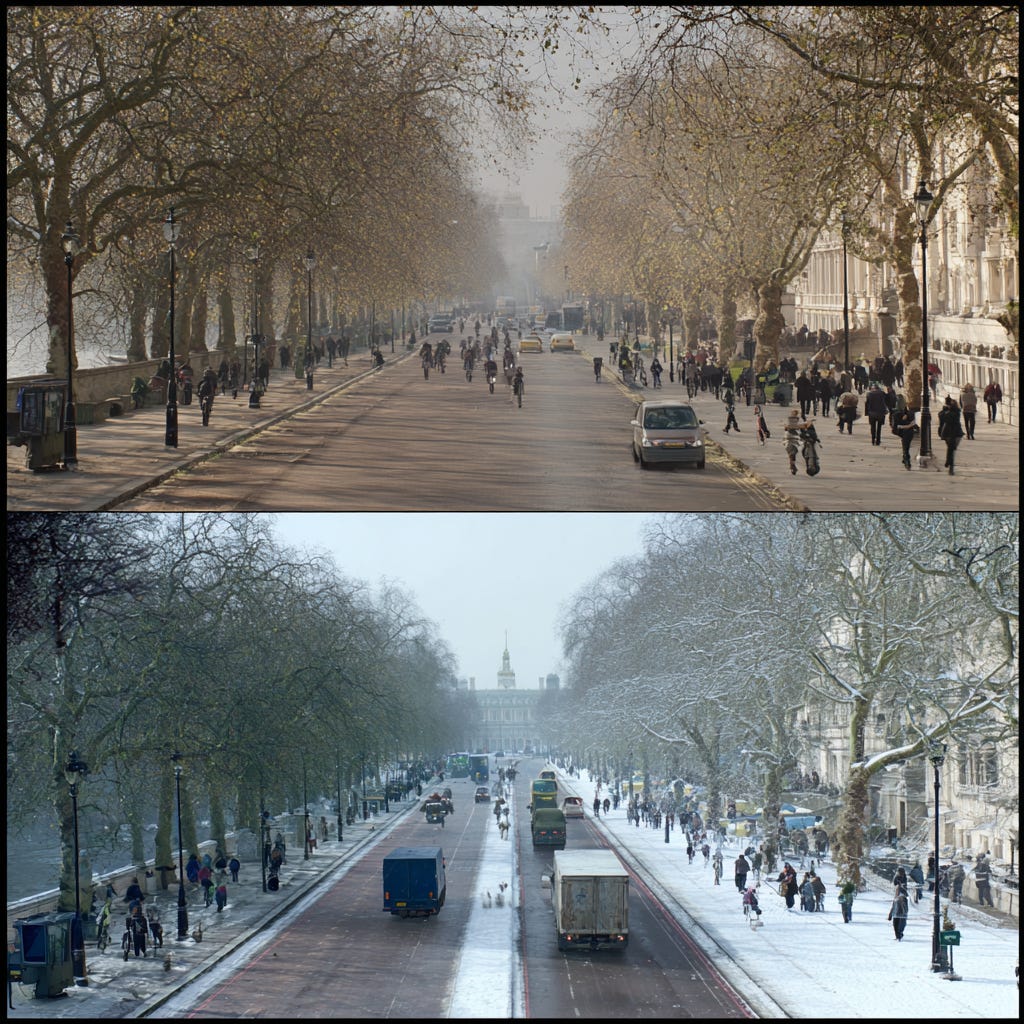
A vision model trained on London’s summer mornings can start losing confidence by November. The city turns reflective; to the human eye, the scene is still London, but to the model, it’s an entirely new world. This is drift, not a server crash, not an obvious bug, but a quiet decay that begins the moment the world changes faster than the model can keep up.

Machine learning systems rarely fail overnight. Their decline is gradual, almost imperceptible. The model keeps running and predictions keep flowing, yet beneath the surface, a silent divergence grows between what the model remembers and what it sees. Over time, what began as a few misclassifications on a foggy morning can grow into systemic misjudgement, not because the model failed, but because London moved on, and the model didn’t.

What exactly is Drift?

At its core, drift is the degradation of model performance caused by a divergence between the production and training environments.

It can emerge from anywhere — new camera sensors, shifting seasonal light, or evolving user behaviour. Every model begins life as a frozen snapshot of the world; drift begins the moment the world moves on.

Formally, drift describes the divergence between the joint data distributions seen during training and those encountered in production:

\(P_{\text{train}}(X, Y) \neq P_{\text{production}}(X, Y)\)

This joint distribution can be decomposed into two components:

\(P(X, y) = P(y \mid X) \cdot P(X)\)

So drift may occur in either the input distribution P(X) or the conditional relationship P(y∣X), or both. This gives rise to the main categories of drift observed in machine learning systems.

Types of Drift

Covariate Drift (Data Drift)

The input distribution P(X) changes, while the relationship P(y∣X) remains constant. Imagine a CCTV model trained on bright summer mornings in Oxford Street. By winter, the same scene has now changed. The objects haven’t changed, but the way they appear has.

That’s covariate drift, when the visuals change, but the meaning doesn’t.

A time-dependent version, known as temporal drift, happens when input data varies by hour, season, or event. Morning traffic in London looks nothing like midnight traffic. Unless the model encodes these rhythms, performance will fluctuate with time.

Prior Probability Drift (Label Drift)

The overall class or label distribution P(y) changes, even if the inputs look similar. In summer, London’s roads are full of cyclists (y1) and people (y2). Your model is trained on this “normal” distribution P_train(y). In winter, there are far fewer cyclists but a surge in delivery vans (y3). The model’s idea of a “normal” scene is now wrong. It may become over-confident in predicting cyclists (its prior) and less accurate at identifying the newly common vans. This shift in balance is label drift.

This is a critical factor for models sensitive to class imbalance.

The frequency of what you are trying to find changes, even if the inputs and meanings stay the same.

Concept Drift

The mapping between inputs and outputs P(y∣X) itself changes. The same input now implies a different meaning. A content moderation model is trained to X (a “thumbs up” gesture) as y1 (”benign”). The company expands to new regions where this gesture is offensive. The human labelling team is now retrained to label the same X as y2 (”offensive”). If the model isn’t retrained, it will fail, a victim of concept drift.

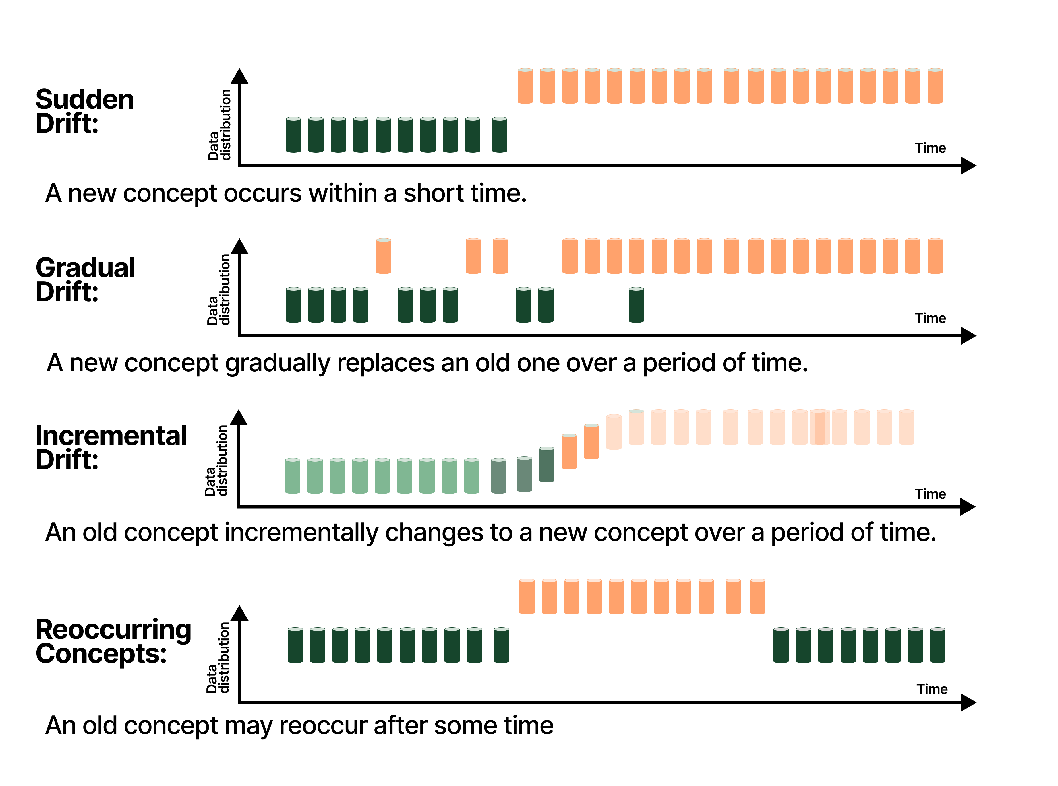
Concept drift can occur in several ways:

Sudden Drift: An abrupt change in rules or context.
Gradual Drift: A slow evolution over time.
Incremental Drift: A sequence of small, cumulative changes.
Recurring Drift: Old patterns re-emerge cyclically.

Concept drift happens when the meaning of the data changes, but the model keeps seeing it the old way.

Model Obsolescence & Internal Factors

Not all decay comes from data. Some arise within the model itself and are operational, not statistical. This isn’t drift in the strict sense, but staleness as the model stops keeping pace with a changing world. The clearest form is Algorithmic Obsolescence, where architectures or representations age out. A CNN, once state-of-the-art, may falter against newer vision transformers, not because the data changed, but because the model didn’t evolve. As data evolves, weights and hyperparameters tuned for past distributions gradually reflect drifts. This form of decay highlights that a model is an artefact of its time.

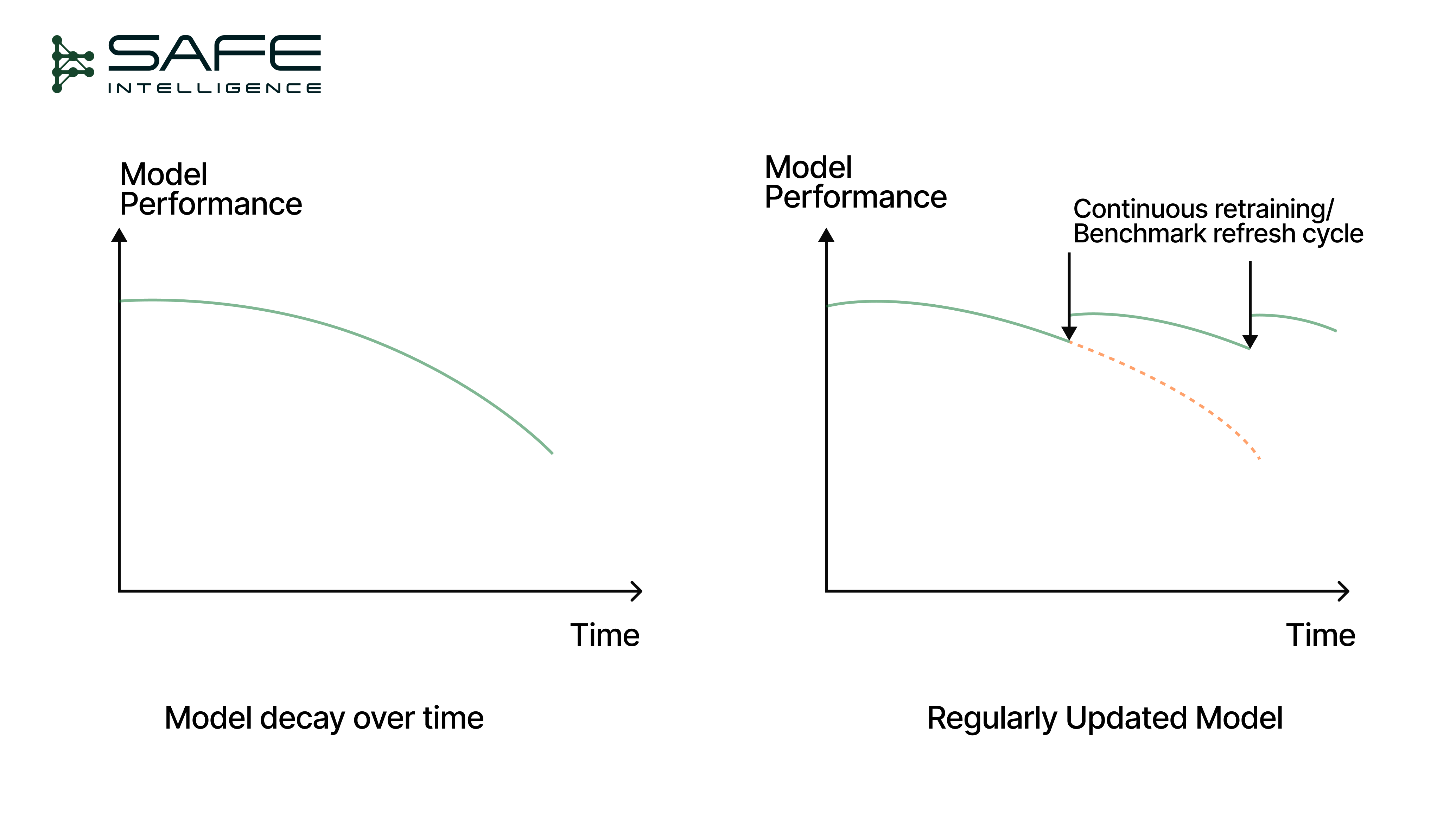
This is why continuous retraining pipelines and benchmark refresh cycles are critical MLOps practices, as they provide a mechanism not only to update data but also to upgrade the model’s architecture and training methods periodically

Drift in Computer Vision Systems

In computer vision, drift isn’t abstract, but it’s visible. A model’s perception of the world depends on light, texture, and hardware, so even subtle changes can disrupt its understanding. Data drift occurs when the pixels themselves change: new camera sensors or image processors alter colour balance and noise; compression or resizing in production reduces image fidelity; and seasonal light alters how edges and shadows are captured. The world looks the same to us but differently to the model.

Concept drift is more deceptive. The pixels stay the same, but their meaning shifts. A product classifier for “shoes” may fail when confronted with new designs it was never trained on. A defect detector once accurate for “scratches” and “dents” may struggle with a new category, such as “micro-fractures.” In other cases, the ground truth itself evolves; for instance, content moderation models must constantly adapt as community standards redefine what is considered unsafe.

The MLOps Playbook on How to Monitor Drift

You can’t detect change without a baseline, and monitoring is not a passive activity but an active statistical process. rift detection begins with a reference. A baseline profile captures the statistical fingerprint of your training data with histograms, quantiles, mean, and variance for numeric features; category counts for discrete ones. For vision systems, this is the most critical step. Drift cannot be tracked at the pixel level; instead, you monitor:

Proxy Metrics: Distributions of low-level features like brightness, contrast, and sharpness.
Embedding Distributions: The statistical profile (e.g., mean, covariance, or a learned density model) of embeddings extracted from a frozen backbone (e.g., ResNet or ViT).

This baseline becomes the “ground truth” against which all future data is compared. With a baseline established, data drift monitoring uses statistical tests to assess how new data deviates from the baseline.

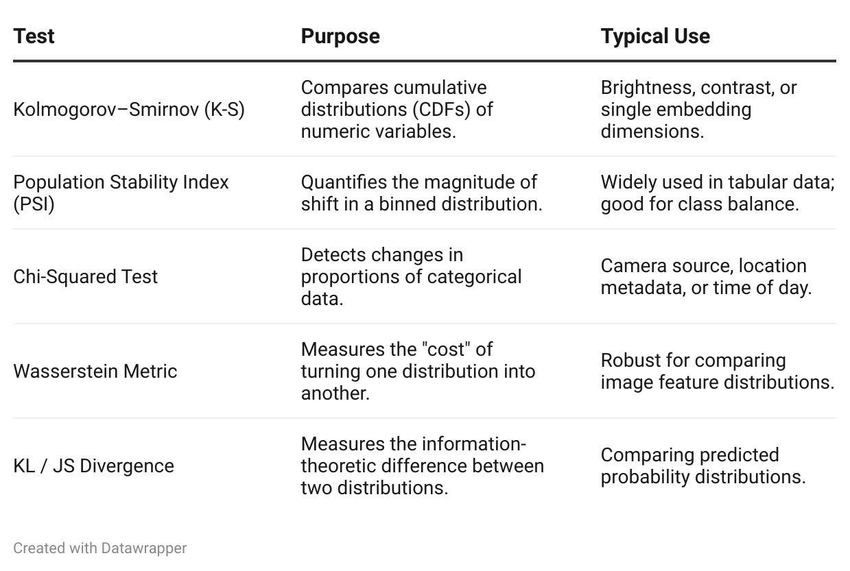
Statistical Distance Methods (for Low-Dimensional Proxies)

For 1D proxy metrics (like brightness) or categorical features, classical statistical tests are highly effective and explainable.

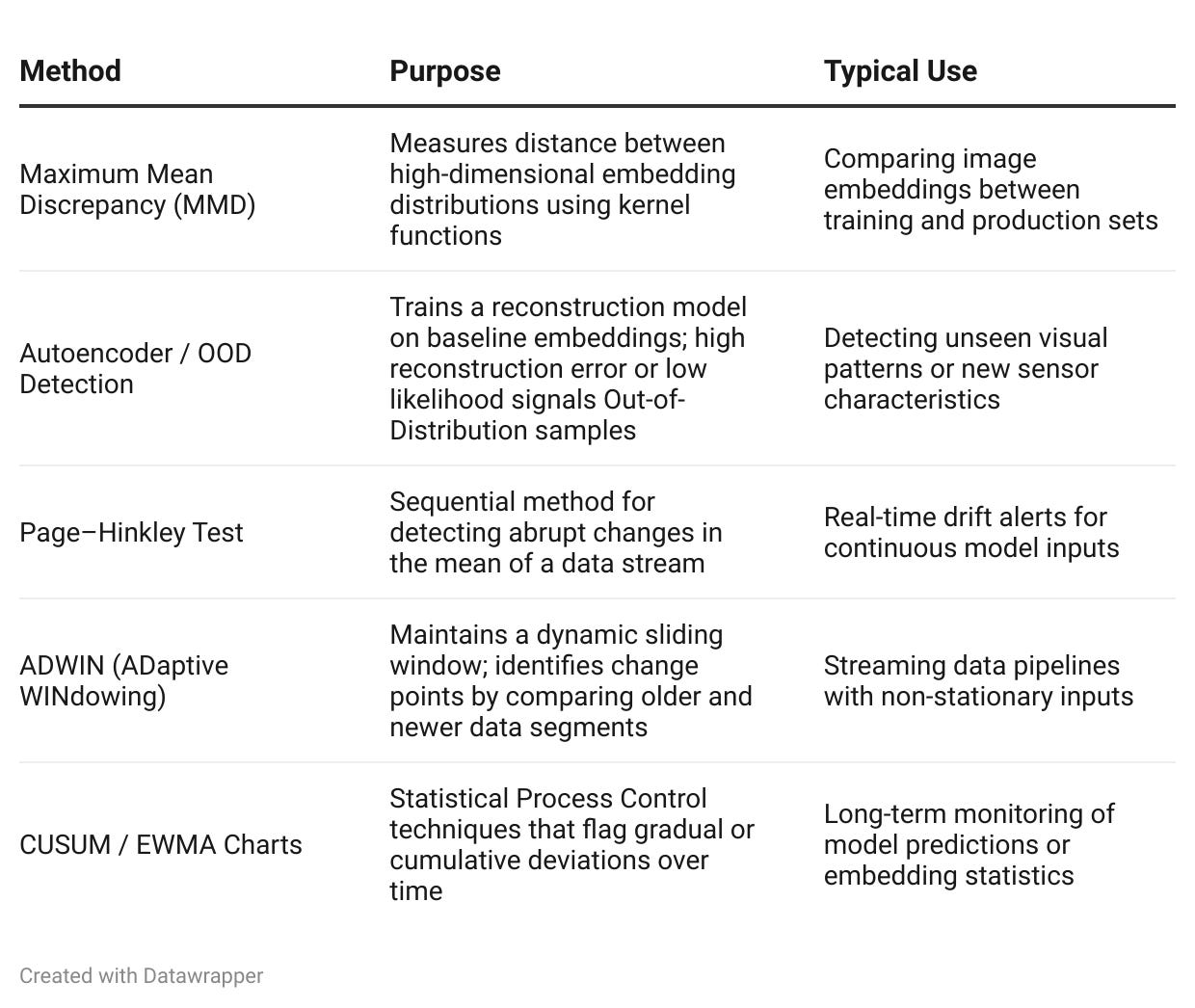
High-Dimensional and Streaming Methods (for Embeddings)

Classical tests lose power in high-dimensional embedding spaces. For this, more advanced methods are required.

Monitoring Concept Drift

Concept drift is the hardest to monitor because it concerns meaning, not just data. Detecting it requires ground-truth labels, which in production are often delayed, sparse, or expensive. When labels aren’t immediately available, monitoring must rely on indirect signals.

Without Labels (Indirect Monitoring)

In the absence of new labels, the most practical approach is to observe the model’s own behaviour. Track the distribution of predictions over time: if a model that once predicted [80% A, 20% B] now outputs [50% A, 50% B], its internal representation of the problem has shifted. Similarly, monitor confidence entropy; a rise in uncertainty or wider spread of confidence scores often precedes measurable accuracy decay. These indicators don’t prove drift, but they are early warnings that the relationship between inputs and outputs may have changed.

With Labels (Direct Monitoring)

When ground truth becomes available, drift detection becomes concrete. Track performance metric over rolling windows to reveal gradual degradation. To separate real decay from random noise, apply Statistical Process Control (SPC) techniques, such as EWMA or CUSUM charts, which flag statistically significant performance drops. The most reliable systems maintain a human-in-the-loop, continuously labelling a small, rotating sample of production data (typically 1–2 %). This rolling ground truth acts as a living benchmark, enabling early detection and timely retraining.

In practice, effective concept-drift monitoring combines indirect statistical signals for speed with direct labelled feedback for certainty, closing the MLOps feedback loop between data, model, and meaning.

Key Takeaways

Building a high-performance model is not the finish line, but a starting point. The real challenge in production machine learning is keeping models relevant and resilient to the inevitability of change. Here are the key takeaways for building a drift-robust MLOps practice:

Monitoring Is Not Optional: The world will change, and your data will change with it. Continuous monitoring isn’t an add-on but a core requirement for any deployed model. Use a defence-in-depth strategy that includes statistical tests, embedding-level methods, and performance metrics.
Detection Without Response Is Just Noise: Every alert must lead to action. Adaptation strategies fall into two complementary paths:
- Data-Centric Mitigation: Fix the data. Use data augmentation to simulate new conditions (e.g., fog, lighting, sensor noise) or active learning to re-label uncertain or drifted samples.
- Model-Centric Mitigation: Fix the model. Choose full retraining for maximum reliability, incremental fine-tuning for speed, or online learning for continuous, real-time adaptation.
Close the Loop: Drift is an engineering problem; monitoring pipelines must be automated to trigger alerts, and those alerts must connect directly to governance and retraining workflows.
Keep Recalibrating: Treat your model like a camera that must be constantly refocused and recalibrated to keep seeing the world clearly. The goal is not a perfect model, but a resilient one.