

Validation Begins with Test Design
Why Your Test Set Is More Than Just a Data Split

Table of Contents
Test Set Design Techniques
TL;DR
Hey there, welcome back to the series. In the last post, we talked about why testing machine learning (ML) feels more like uncertain geology than precise geometry. This piece builds on that, arguing that real model validation—the process that makes a model truly ready for the real world—doesn't start with chasing a high performance score. Instead, it begins with deliberately designing your test sets. A test set is more than just the data left over after training. Real confidence comes from strategically engineering your test data to be a tough, real-world simulator that actively seeks out your model's breaking points.

“All models are wrong, but some are useful.” – George E. P. Box
No matter how advanced techniques become, every ML model remains inherently an approximation of reality. Recognising this essential limitation sets the context for why rigorous validation is not merely desirable but indispensable. This inherent imperfection raises the critical question: How good is good enough? The answer lies in building confidence, specifically, confidence that the model will reliably perform as intended in real-world operational conditions. This essential pre-deployment confidence is forged through validation.
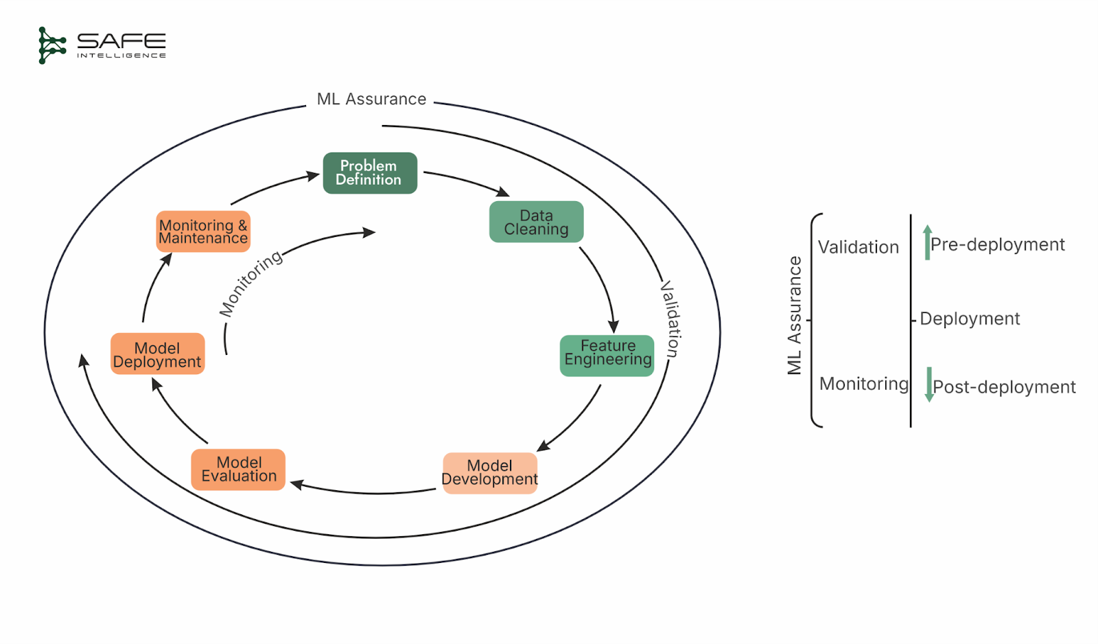
Validation is a comprehensive assessment of all aspects of a model’s design, development, and final performance to ensure its readiness for deployment. Within this validation framework, two distinct technical processes are critical: testing and verification.
Testing involves running inference on curated datasets to evaluate model performance against specific, predefined criteria in the scope of supervised learning.
Verification, briefly introduced here but to be explored in detail in a later part of this series, uses formal mathematical methods to prove or establish high confidence in critical properties.
Before continuing, let's clarify our scope. In this series, we define validation as the technical, pre-deployment assurance process. While some include monitoring or governance under this umbrella, we treat them as separate concerns (post-deployment assurance). Validation focuses strictly on testing and verification that determine whether a model is ready for deployment.
Getting Test Set Design Right
A test set is not just a leftover slice of data, nor is its worth measured by size or a single performance score. Its fundamental purpose is to expose whether a model is truly deployment-ready by surfacing the necessary vulnerabilities. To achieve that, a well-designed test set rests on four pillars: representativeness of the production environment, exhaustive coverage of mission-critical use cases, targeted probes that hunt for hidden failure modes, and strict isolation from training data to preserve evaluation integrity.
Representativeness
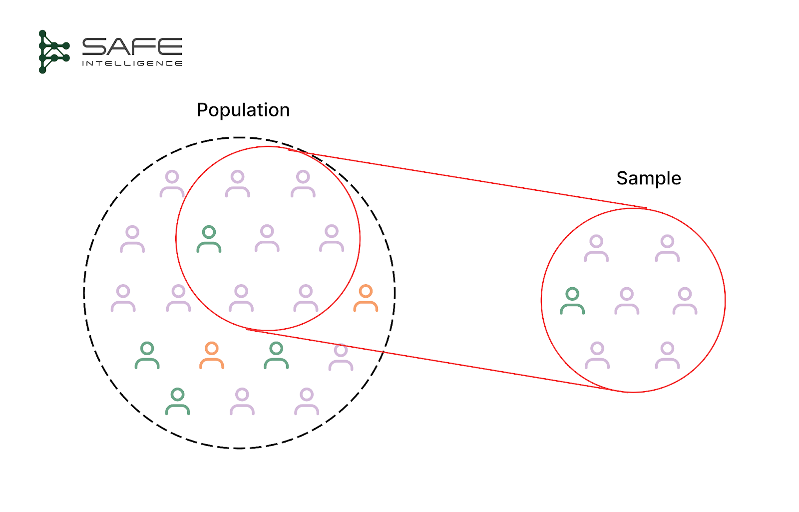
A test set must resemble the world the model is about to enter so that its metrics give an unbiased, deployment-ready performance estimate. This demands disciplined sampling: include every region, population, or channel the model will encounter; balance rare but critical classes to avoid optimism that hides failure; and, when data are scarce, augment the training pool with synthetic examples so real-world instances can be reserved for evaluation. Furthermore, representativeness is temporal; a test set built on year-old data is a poor proxy for today's reality.
Coverage
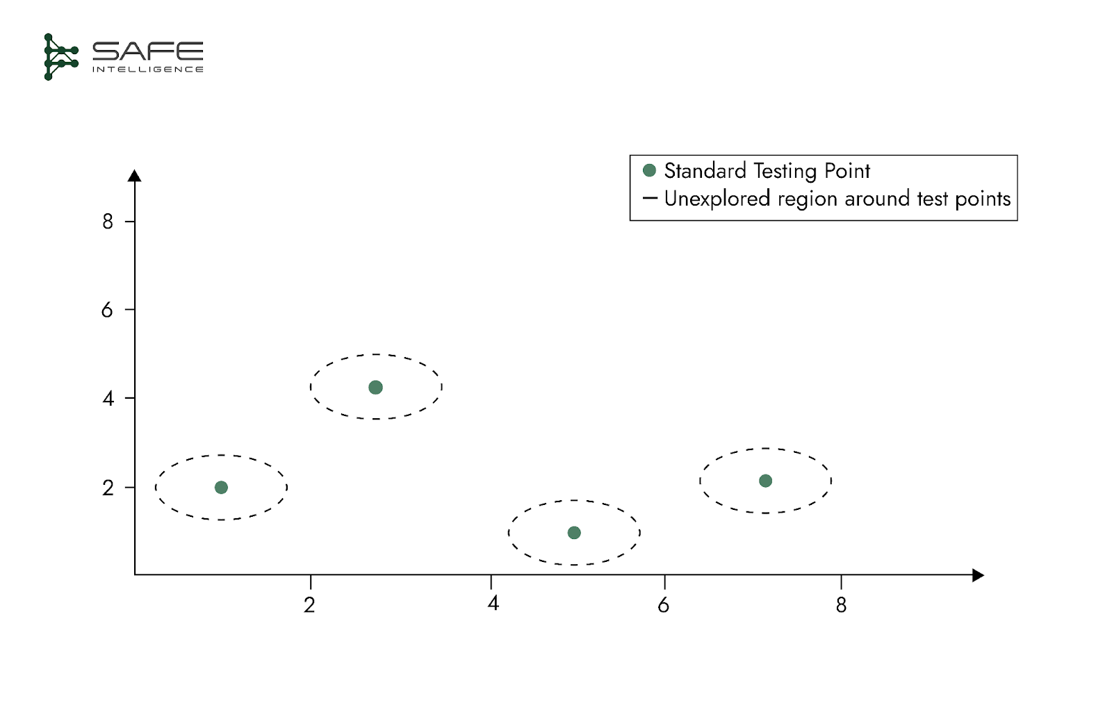
Typical test sets evaluate model performance at discrete data points, leaving vast, unexplored regions around these points. Models may appear highly performant at isolated test points yet fail significantly when slight variations occur. Therefore, robust test design must encompass broader regions around key test points, ensuring performance stability across relevant data neighbourhoods.
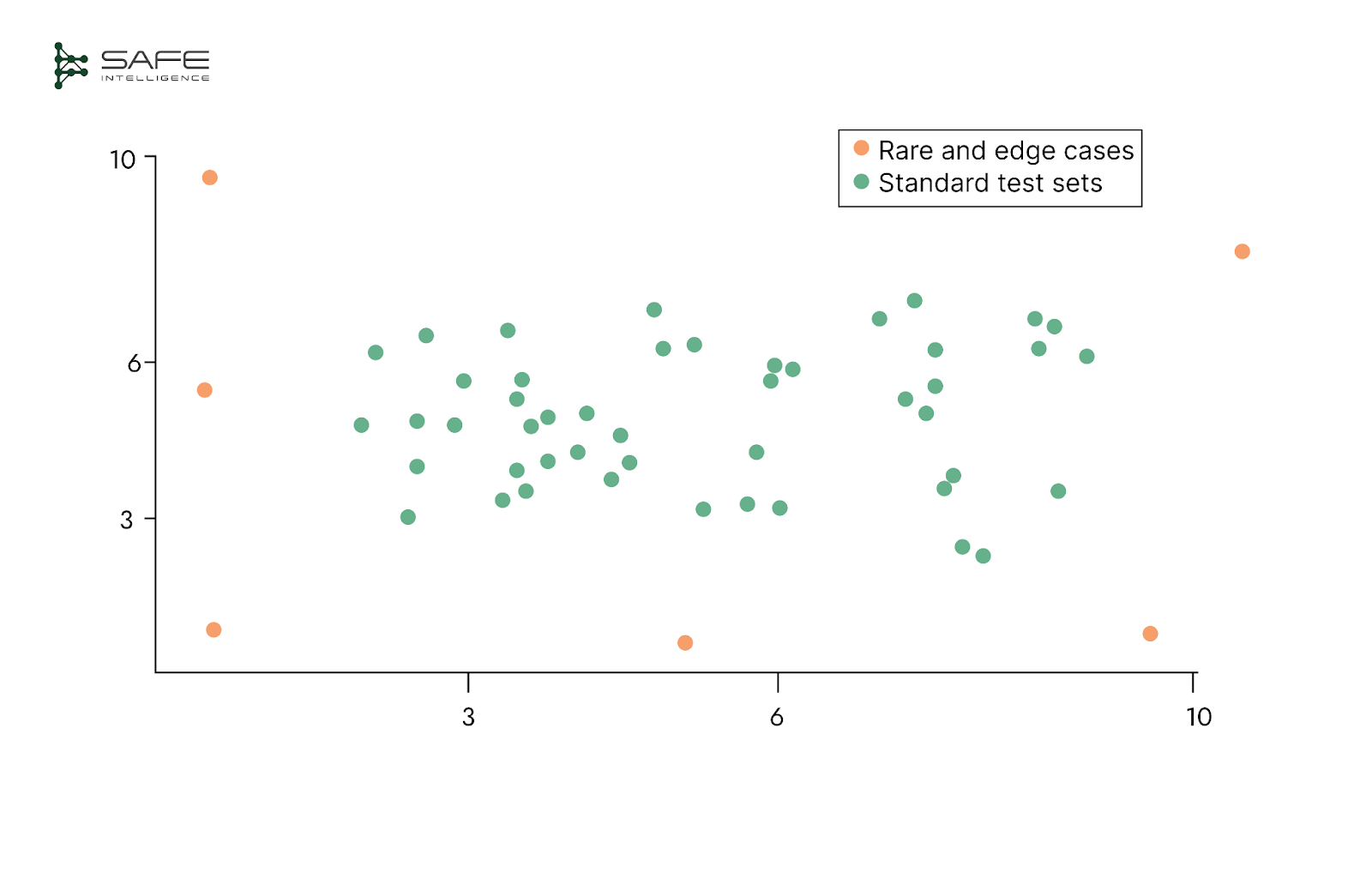
A well-designed test set must go far beyond the “happy-path” cases where a model is already comfortable. It should deliberately sample the whole operational landscape, cutting across routine inputs and the rare, high-impact situations that can break a system. Work with domain experts to inject boundary conditions, edge cases, and infrequent but costly events (e.g., large fraud attempts). Slice scenarios by real-world stressors such as peak load and holidays—so you see how performance shifts when the stakes are highest. Only this breadth of coverage reveals whether the model is ready for production.
Probes for Model Failure
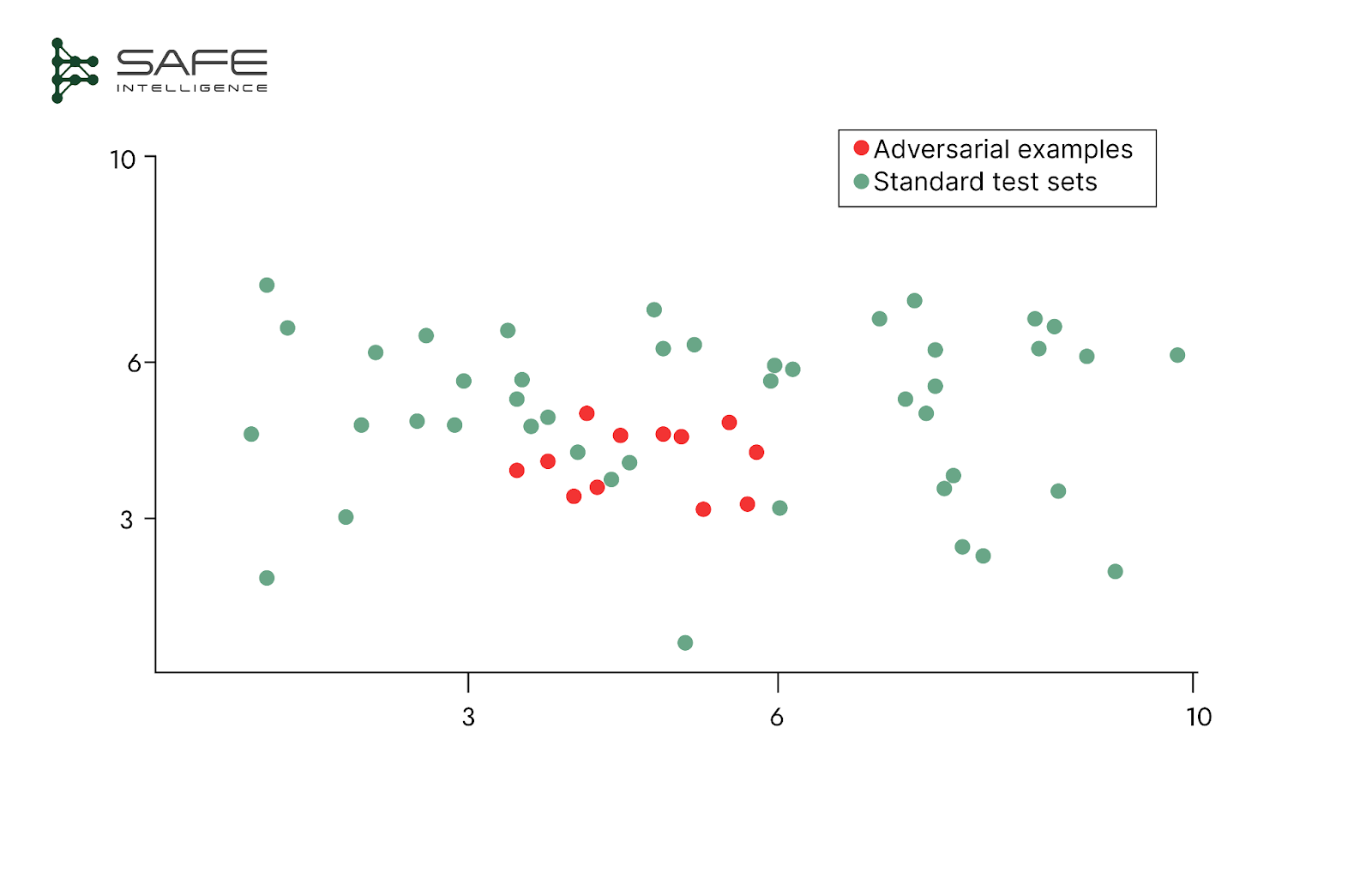
An effective test set must actively probe for model failures, not just confirm the model works. This requires designing specific inputs to uncover hidden weaknesses and logical inconsistencies. One approach is behavioural testing, where we verify the model's reasoning: does its output remain correctly unchanged when an irrelevant input is modified (invariance), and does it change predictably when a relevant one is adjusted (directional expectation)? The other approach is stress testing for stability, assessing performance on inputs with real-world imperfections like poor lighting, out-of-focus images, or noisy data. The most rigorous form of this is adversarial testing, which uses inputs carefully crafted to find a model's breaking points. If a test set never challenges the model, you’re not truly validating; it’s just performance theatre.
Maintain Strict Evaluation Boundaries
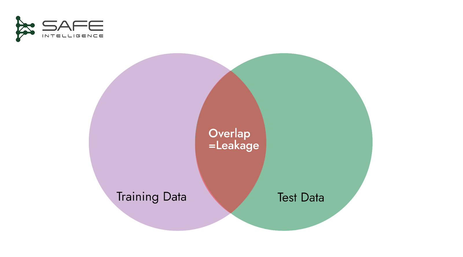
Isolation is non-negotiable; partition the test set at project inception, lock it away, and never let it contaminate training or model-selection steps. This absolute separation prevents all forms of data leakage, from direct sample overlap to subtle information bleed through proxy variables or shared preprocessing artefacts. Ultimately, this disciplined isolation is the only way to guarantee that the test set provides a true, unbiased measure of generalisation performance, ensuring you evaluate a model's ability to perform on unseen data, not merely its memorisation capacity.
Test Set Design Techniques
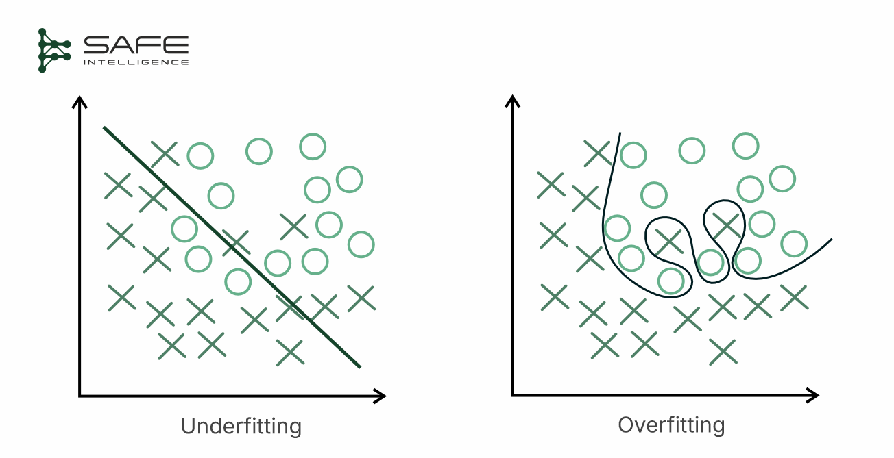
While the principle of isolation demands a strict separation of test data, the method of this separation is a critical design decision. A poorly chosen split can introduce high bias (underfitting), leading the model to oversimplify, missing important complexities in real-world data, or, conversely, high variance (overfitting), causing the model to memorise specifics rather than general patterns. Although it appears accurate during training, it performs poorly on new, unseen data.
Test set design is not an afterthought; when crafted efficiently, it drives the model toward genuine production readiness and gives stakeholders evidence they can trust. That rigour starts with how you carve raw data into a training slice for model building and an isolated slice for evaluation. Below are the principal splitting strategies:
Simple Data Split
A straightforward way to partition your data for training and evaluation is by using either a train–test or a train–validation–test split. In the latter, a validation set is specifically used for hyperparameter tuning, model selection, and iterative improvements, while the test set is held out until the very end for a final, unbiased performance check.
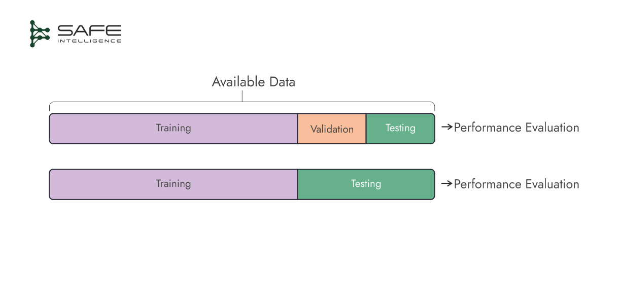
A common split ratio is 70% training, 15% validation, and 15% test. If you only need a high-level performance estimate, a 70–30 train–test split can suffice.
Cross Validation Techniques
While a simple data split is easy to implement, it can yield unstable or biased estimates, particularly if your dataset is small or not representative of the underlying distribution. Cross-validation overcomes these limitations by repeatedly training and evaluating the model on different subsets, offering a more robust view of how it will perform on unseen data. Crucially, every portion of the data is used for training and validation/testing at some stage, leading to more comprehensive performance metrics. Although cross-validation requires multiple training runs and can be computationally expensive—especially for large datasets—it often provides more reliable insights into real-world performance. It is especially valuable when you have limited data, allowing you to maximize both training and evaluation opportunities. Let’s look at some form of cross-validation:
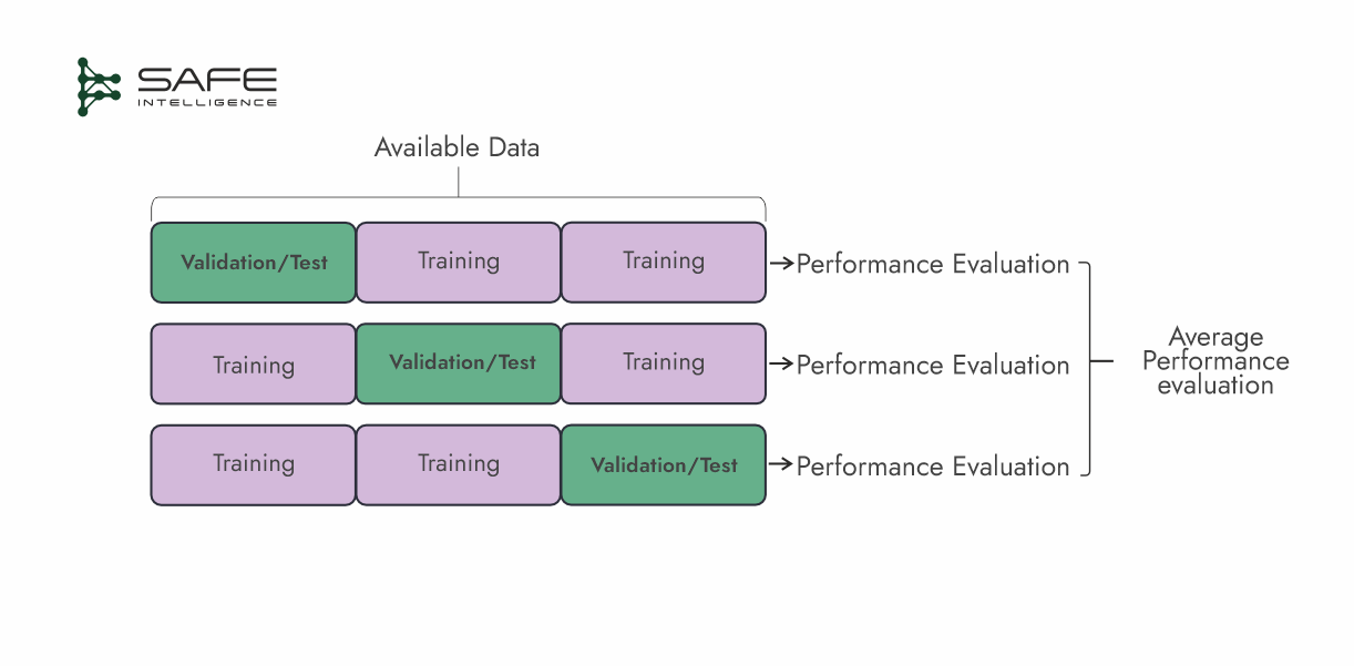
k-Fold Cross-Validation
This cross-validation strategy splits the dataset into ‘k’ roughly equal ‘folds.’ In each of the k iterations, one fold is used as the validation/test set, while the remaining folds are used for training. Performance metrics are average over the k-folds for a more stable estimate
Repeated k-Fold Cross-Validation
This strategy involves performing k-fold cross-validation multiple times with different random splits. This approach further reduces variance in the performance estimate by averaging results across all runs. The ‘k‘ here doesn’t mean the number of folds but represents the number of times you repeat the entire training–validation process with different random splits.
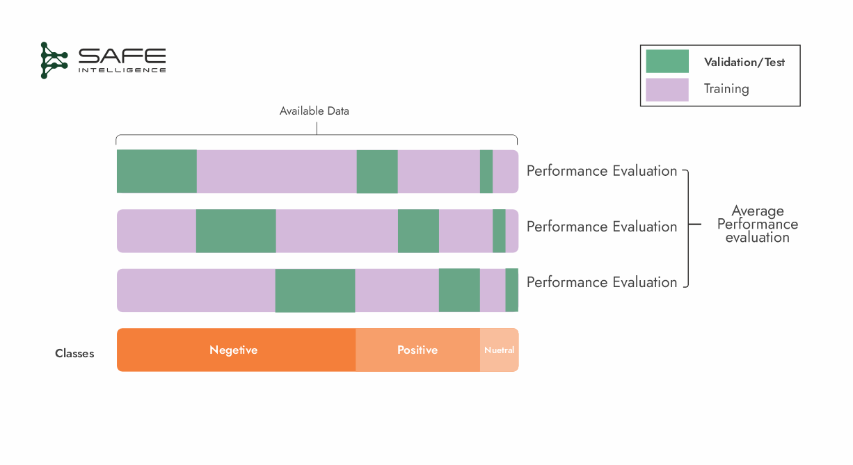
Stratified k-Fold Cross-Validation
This strategy is a variant of k-fold cross-validation, where each fold is created in a way that preserves the overall class distribution. In simple terms, if you have an imbalanced dataset with the target of 60% negative, 30% positive, and 10% neutral, each fold will aim to have roughly 60% negative, 30% positive, and 10% neutral samples. If you simply shuffle your data randomly, there is a chance that one fold may end up with more positive samples than another. Stratified k-fold tries to avoid that, as data imbalance can skew how you measure performance. Stratification ensures that every fold reflects the true proportions of each class (like a mini version of the full dataset).
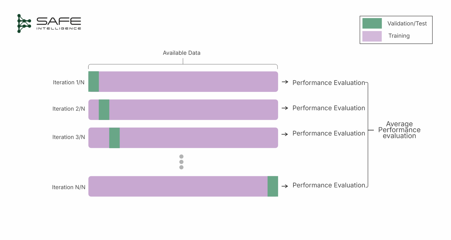
Leave-One-Out Cross Validation (LOOCV)
Leave-one-out cross-validation (LOOCV) is a case of k-fold where k equals the number of data points (n). Each iteration uses one sample as the test set, while the remaining n-1 samples form the training set. A model is trained on these n − 1 samples and validated on the single held-out sample. This procedure is repeated n times—once for each data point as the test set—and the final performance metric is the average across all iterations. This maximizes your data for training, often leading to lower bias in the estimate. Training the model n times can be extremely computationally expensive, especially for large datasets. Leave-p-Out Cross-Validation (LpOC) generalizes LOOCV by leaving out p samples instead of one. This strategy requires training on all remaining data points for each possible selection of p samples, and it is still computationally intensive.
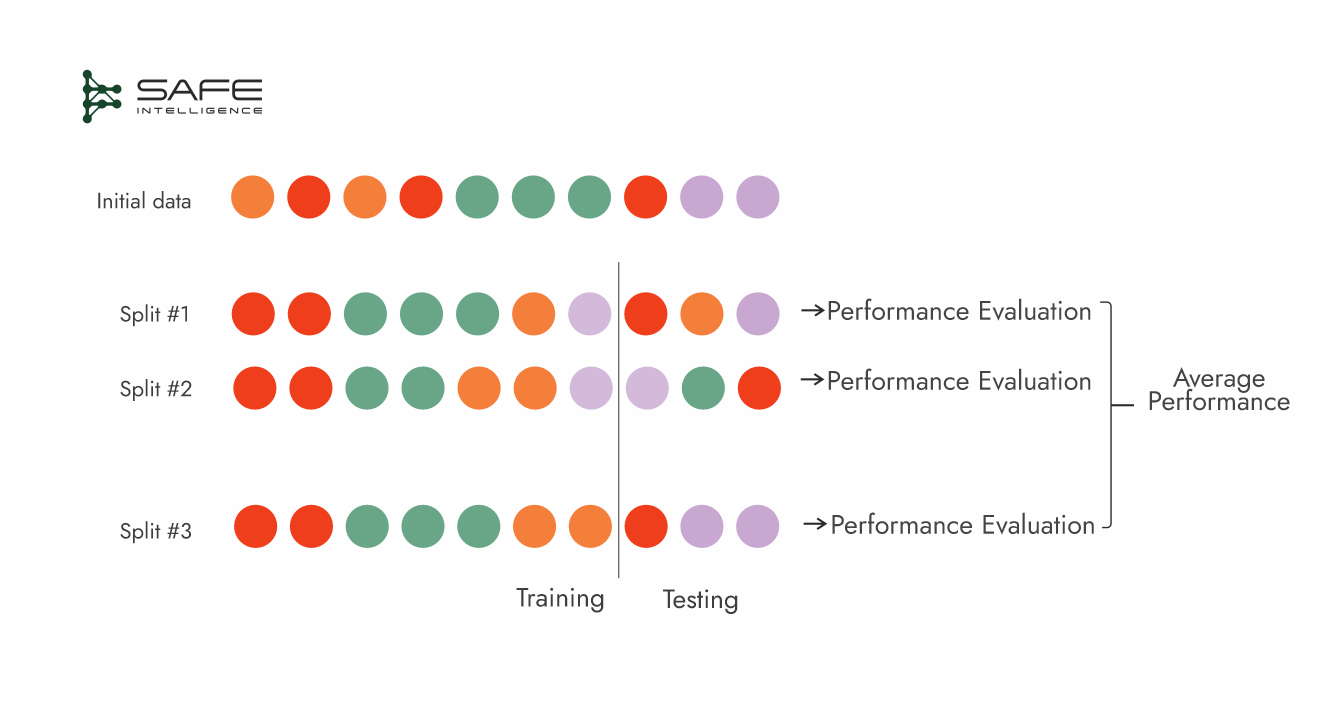
Monte Carlo (Repeated Random Sub-Sampling) Cross-Validation
Monte Carlo cross-validation creates multiple, independent train-test splits by repeatedly sampling the data at a fixed, predefined proportion (e.g., 70:20). For each split, a new model is trained from scratch and evaluated, with the final performance metric being the average across all iterations. While highly flexible, this method's primary trade-off is its lack of guaranteed coverage, as some data points may be tested multiple times while others are never selected for a test set at all.
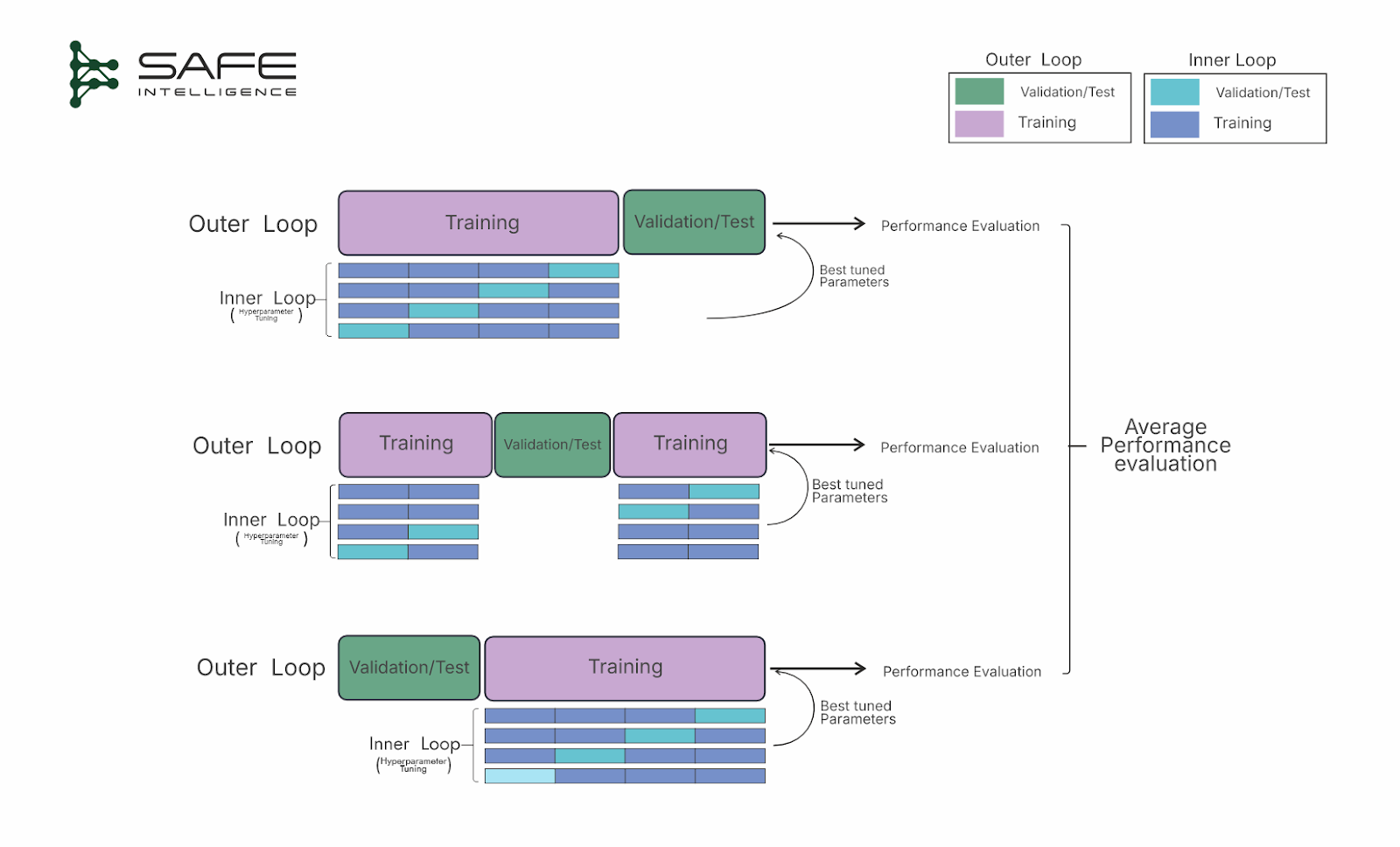
Nested Cross-Validation
Using the same cross-validation procedure and dataset for both tuning and final evaluation can result in overly optimistic and biased estimates. Nested CV aims to prevent this by embedding one cross-validation loop within another to prevent information leakage between hyperparameter tuning and performance assessment. To avoid this, the outer loop splits the data into k folds, designating a fold(s) as the test fold and the remaining folds for training. Inside each outer training set, an inner loop performs its cross-validation purely for hyperparameter tuning, selecting the best model configuration. The tuned model is then evaluated on the outer test fold. This process repeats for each fold in the outer loop, and the results are averaged to provide an unbiased performance estimate. Although more computationally demanding, nested cross-validation is invaluable for reliably comparing models and hyperparameter settings.
Time series Cross-Validation
These cross-validation strategies are designed to respect the chronological order of data, ensuring that only past observations are used to predict future outcomes. Two main approaches are a sliding window and an expanding window. In the sliding window approach, a fixed-size window of the most recent observations is used for training, then the window shifts forward to discard older data and include new arrivals. This strategy keeps the model focused on recent trends but may lose potentially useful historical information. Conversely, the expanding window method starts with an initial set of observations and grows over time, retaining all prior data. While this strategy preserves the full historical context, older data might become less relevant, and the training set can grow unwieldy.
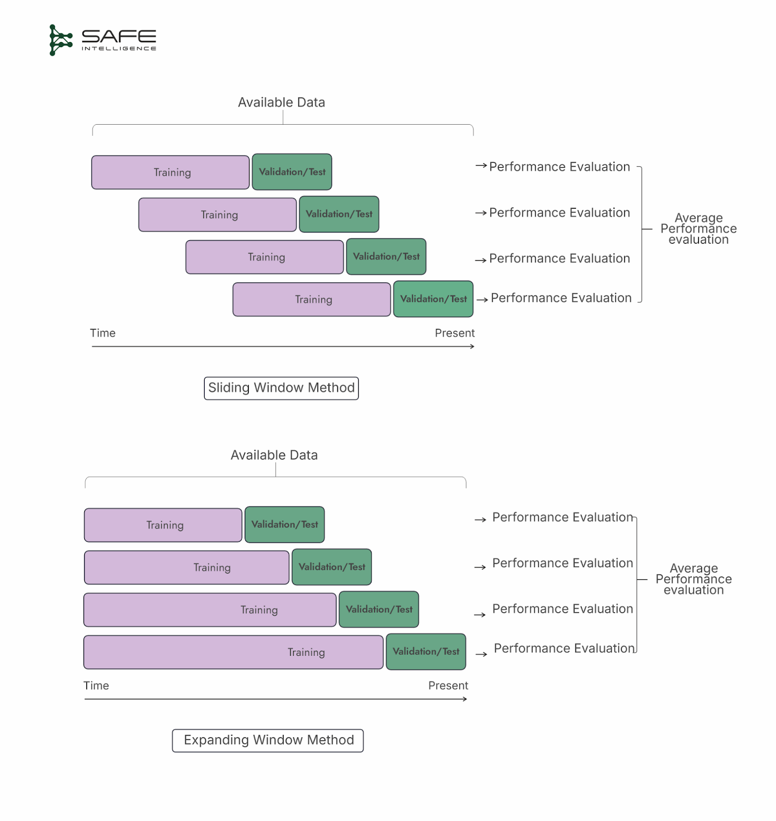
Time series cross-validation simulates real-world forecasting scenarios by providing multiple, chronologically consistent validation points. Additionally, the overlapping training sets can drive up computational costs, particularly for large datasets.
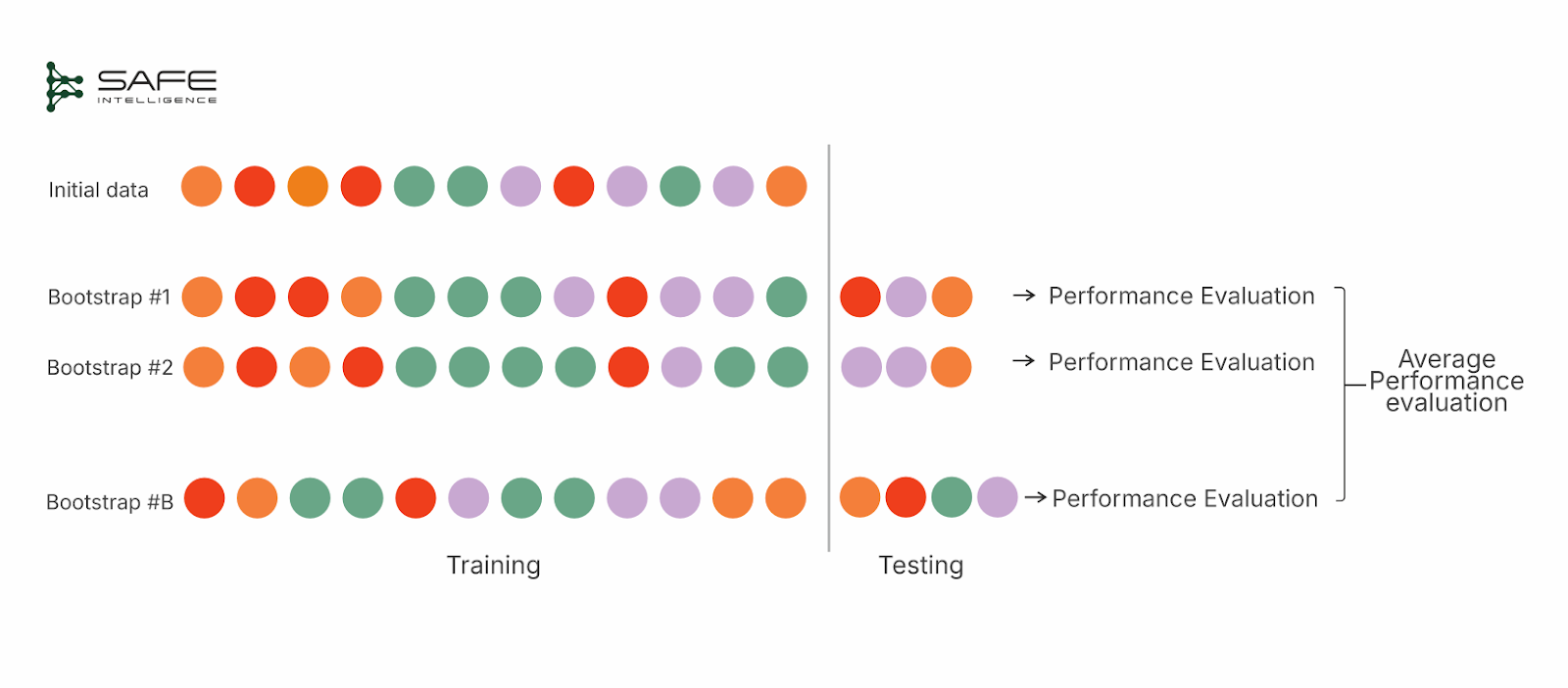
Bootstrapping
Bootstrapping is a resampling method for estimating model performance by repeatedly drawing new training sets with replacements from the original dataset. This strategy simply means each time you pick a data point for training, you place it “back” into the pool so you can choose the same point again in subsequent draws. Each “bootstrap” produces a dataset the same size as the original but with duplicated entries. The out-of-bag (OOB) samples—instances not chosen in that draw—serve as the test set. After multiple iterations, you average the OOB results to estimate performance. Bootstrapping, by contrast, may repeatedly sample certain points while omitting others, which can lead to a bias unless adjusted (e.g., via .632/.632+ methods).
What do evaluation metrics really tell us?
We often prioritise evaluation metrics like accuracy, precision, recall, F1 score, or RMSE when evaluating a model's health. See the Neptune AI guide on performance metrics for an excellent deep dive into how different metrics work and why they matter. However, it's crucial to remember these numbers are merely proxies—indirect measures of a model's true effectiveness in real-world scenarios. This is because direct measurement of real-world impact is often impractical during development; we optimise against these surrogate metrics. But there's an inherent risk: focusing too heavily on optimising these metrics can cause a model to "overfit" to metric specifics, exploiting quirks in training data rather than capturing meaningful generalisable patterns. This pitfall aligns with Goodhart's Law, which states:
"When a metric becomes the target, it stops being a good measure."
Given these limitations, true confidence is forged not in a single score but in the rigour of the validation process itself. This robust approach begins with precise planning, which involves defining the scope of validation—from the data to the final inference pipeline—translating business objectives into explicit, measurable assessments and curating the immutable test sets needed for evaluation. This blueprint is then operationalized within a repeatable validation pipeline to ensure the same standards judge every model. For high-stakes applications, the process is fortified by independent review teams to eliminate confirmation bias, transforming validation from a one-time gate into an iterative cycle of continuously raising the bar for system safety and effectiveness.
Key Takeaways
Validation is the entire pre-deployment assurance umbrella (testing and verification), while monitoring is strictly a post-deployment task.
Design test data for representativeness, broad coverage (including edge cases), explicit failure probes, and airtight isolation.
Evaluation metrics are proxies, not goals. Goodhart’s Law reminds us that over-optimising a single metric corrodes real-world usefulness; confidence comes from a well-governed, repeatable validation pipeline, not a solitary performance score.
Choose the right split strategy to manage bias/variance trade-offs; pick deliberately rather than by habit.
COMING UP… In the next article of this series, we'll explore ML Benchmarking.