

Deploying Machine Learning Models
From Validation to Production


TL;DR
In our last article, we moved beyond conventional testing and introduced formal verification, a deeper form of validation. Now that your model has cleared every validation gate, the next challenge is to deliver it. This article covers choosing the right inference architectures and walks through progressive rollout strategies that aim to minimise risk in high-stakes industries. Lastly, it distils the industry consensus on scaling, which involves standardising, containerising, and orchestrating to handle operational complexities at scale.
Understanding your deployment needs
Before shipping a model to production, step back and map production requirements to the right serving pattern. Four levers drive this decision:
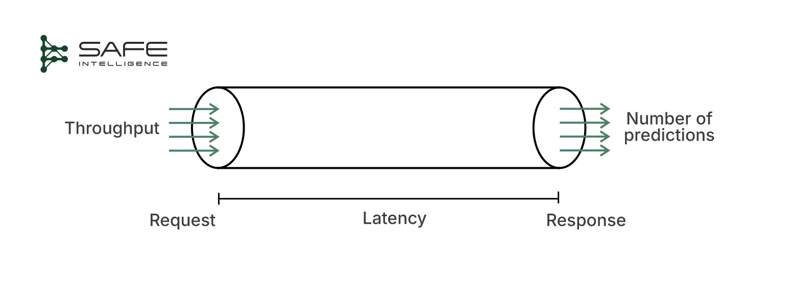
Latency & Throughput: How fast must each prediction return and at what volume? These directly dictate the speed and capacity demands on your system.
Data dynamics: When does input data arrive, and how fresh must predictions be?
Resource constraints & scalability: Available computing power (CPU/GPU, memory) and the infrastructure's ability to scale up or down with varying loads.
Cost & Interaction Model Who/what consumes the predictions, and how price-sensitive is the workload?
Core ML Serving Architectures
With the key criteria in mind, ML models are generally deployed in three main architecture patterns:
Online Real-Time Inference (Synchronous)
Asynchronous Inference (Near Real-Time)
Offline Batch Prediction (Batch Transform)
Each of these has its strengths and ideal use cases. Sometimes different terminology is used (for example, “batch prediction” vs. “offline batch transform” or grouping the first two as both “online” methods, synchronous vs. asynchronous), but the concepts remain consistent. Let’s explore each architecture.
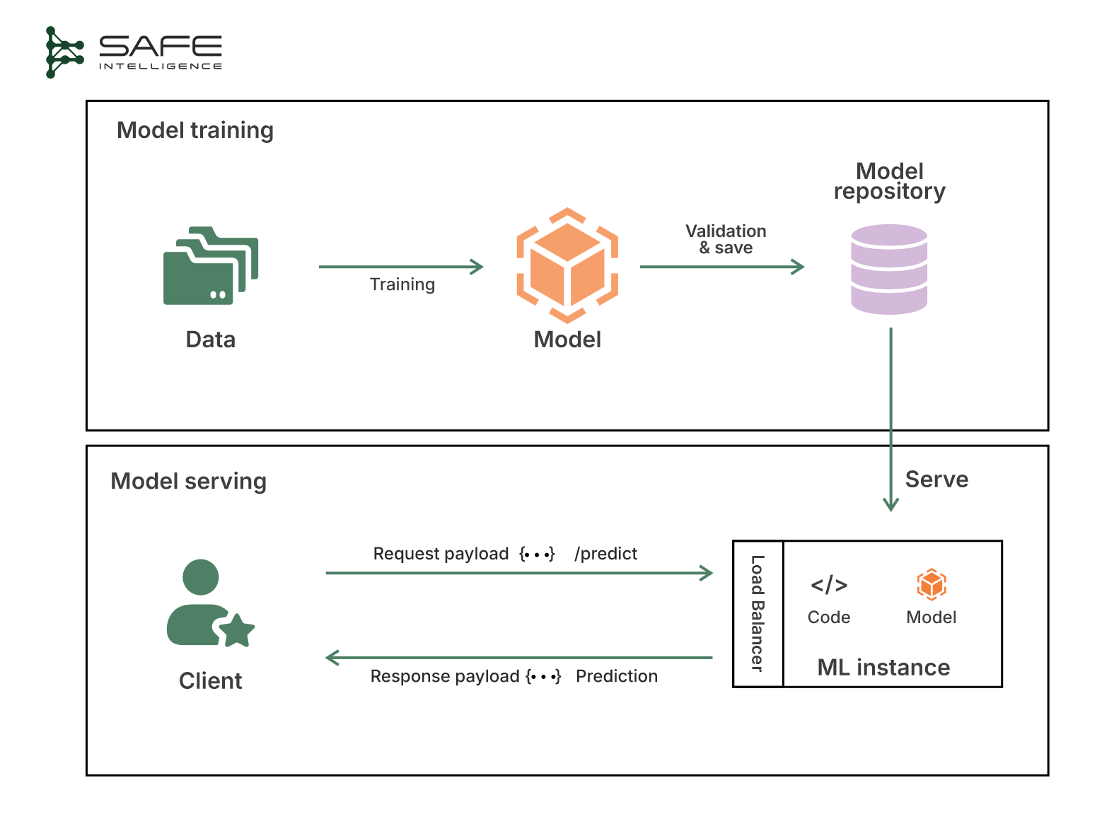
Online Real-Time Inference (Synchronous)
This architecture provides immediate prediction responses with minimal latency. Applications that prioritise speed or interactive responses, like fraud detection at transaction time or cockpit alert systems, find this architecture ideal. Here, the model is served via an API that the users call synchronously (the client sends a request/input and waits immediately for the prediction result). When a request arrives, such as a JSON payload of features, the service loads the model, performs inference, and immediately returns the result. Everything happens within the context of that request, usually in a matter of milliseconds or seconds, as illustrated below:
The system is typically optimised to minimise overhead in response. That might involve keeping models loaded in memory, using fast data stores for features, and even making models lighter or distilling them to run faster. The price of that speed is scalability, such as with more instances or powerful hardware used. Additionally, there is a limit to the throughput achievable with a purely synchronous design; if the request volume exceeds what your servers can handle at the same time, either latency will increase or some requests may fail.
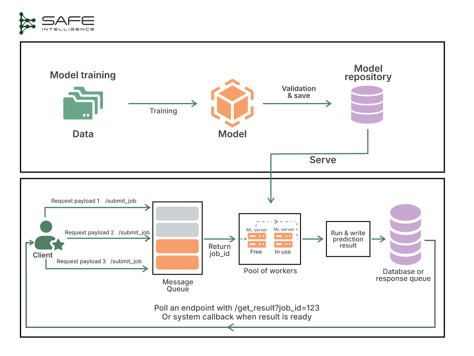
Asynchronous Inference (Near Real-Time)
This architecture addresses the bottleneck of synchronous inference by introducing a message queue between your client and the ML model. The requests are buffered (to absorb bursts), and then stateless workers pull jobs, run inference, and write results to a result store. The client is either alerted or polls a results endpoint to fetch the prediction. Since requests buffer, workers can scale horizontally or even down to zero when idle. The client is either alerted or polls a results endpoint to fetch the prediction. This architecture is illustrated below:
If your latency target is seconds, not sub-100ms, async serving smooths out traffic spikes and converts them into steady, predictable costs while preserving reliability and throughput. Lastly, this architecture provides the avenue to insert preprocessing, enrichment, or post-processing stages directly in the queue flow.
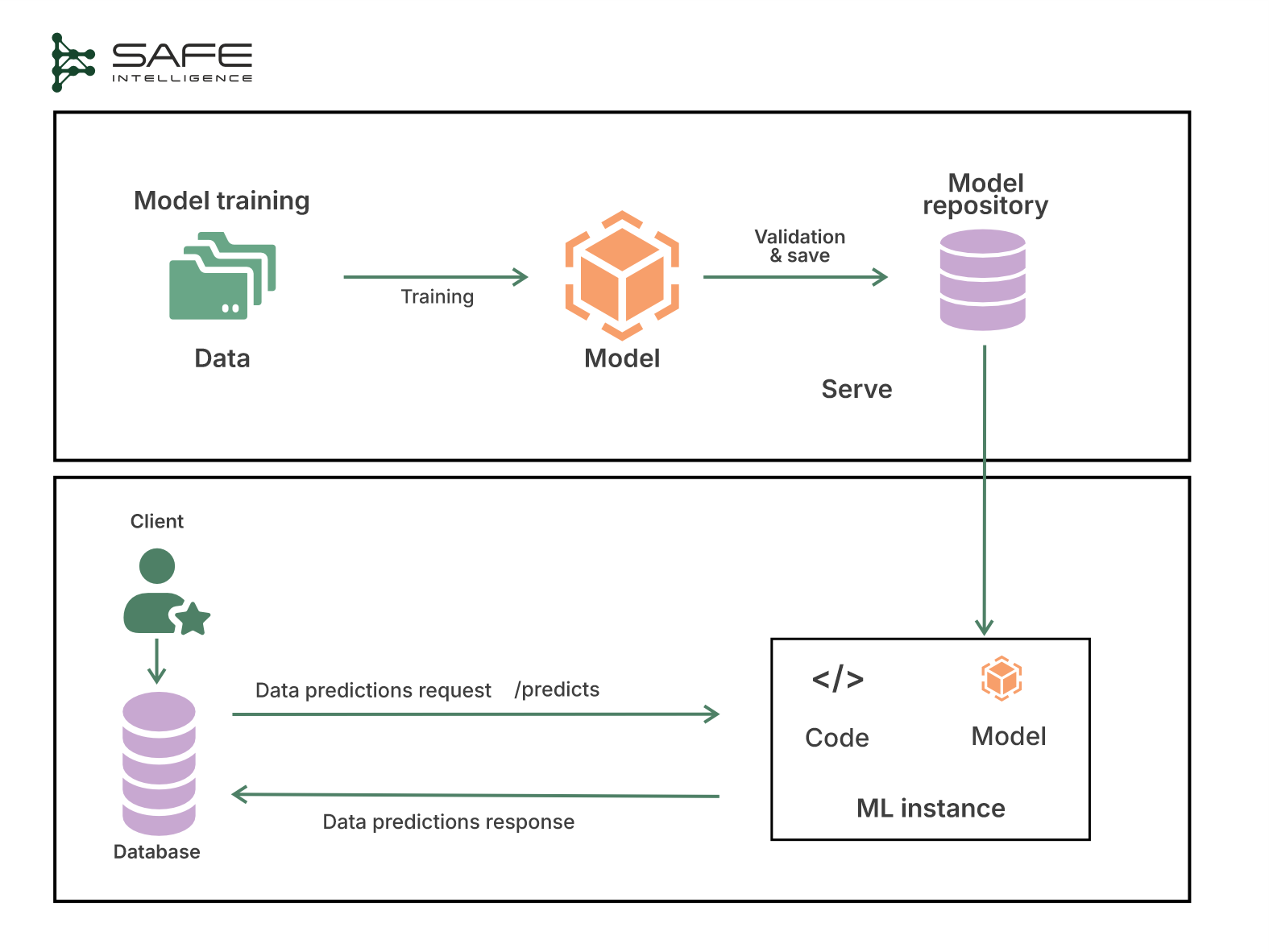
Offline Batch Prediction (Batch Transform)
Offline batch prediction refers to running the model against a dataset slice or entire warehouse on a schedule or trigger and writing the outputs to storage, a data warehouse, or a feature store for downstream use. These batch jobs often run on big data processing frameworks or distributed systems (like Apache Spark, Hadoop, or distributed SQL engines) to churn through huge volumes of input.
By exploiting spot instances and off-peak capacity, you slash costs, and because compute is ephemeral, you never pay for idle GPUs. The catch? Results arrive in minutes or hours, so this is great for back-office analytics but ill-suited to user-facing paths.
Which architecture fits your workload?
Choosing the right inference architecture isn't always straightforward. Use this Q&A-style checklist to guide your decision-making clearly and effectively:
Rollout Strategies: Safely Deploying ML Models in Production
In high-stakes domains like finance and aviation, a “big-bang” model swap (where the old system is shut down and instantly replaced by the new model) is a gamble no one can afford. Modern teams now favour progressive delivery, where new models are rolled out to a small slice of traffic or a safe environment first, validating performance in the wild, then scaling up only when metrics look solid. Let's explore progressive rollout strategies that minimise risk, provide real-world validation, and ensure stability.
Champion/Challenger
In this strategy, you deploy the new model ("challenger") in parallel to the existing production model ("champion"). Both receive the same inputs (mirrored traffic), but only the champion’s predictions directly impact users or operations. The challenger operates in the background, and its outputs are evaluated separately to determine if they outperform the existing model and for other experimental analyses. This is also known as shadow deployment, as the challenger models run in shadow mode (without affecting real outcomes)
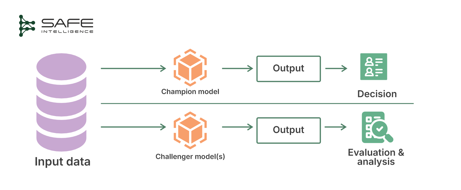
Why choose Champion/Challenger?
This approach is excellent when regulations require proof of model efficacy or when the cost of a bad decision is extremely high. With proper performance and governance analysis over time, decisions on when a challenger is ready to take over as the new champion can be made.
Flask-like pseudocode
@app.route("/predict")
def predict():
    features = request.get_json()['features']

    # Champion makes the actual prediction
    champion_prediction = model_champion.predict(features)

    # Challenger prediction is computed but not returned to users
    challenger_prediction = model_challenger.predict(features)

    # Log challengr results separately for later comparison
    log_to_evaluation_db(features, champion_prediction, challenger_prediction)

    return champion_prediction
Canary deployment
This deployment strategy incrementally deploys the new model to a small fraction of live traffic. The fraction gradually increases this percentage as confidence builds, continuously monitoring performance and stability.
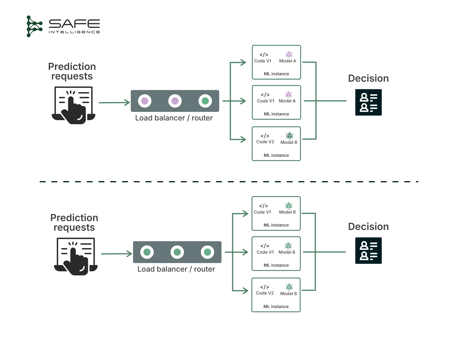
Why choose canary deployment?
Canary deployments are widely used when you want a cautious, data-driven rollout using real traffic. For example, companies like Tesla and Waymo use such rollouts, as they might enable a new vision model for a small set of cars, then expand if it performs well. The canary approach strikes a balance between innovation and caution, swiftly retracting any underperforming model before it causes widespread harm.
Flask-like pseudocode
CANARY_PERCENTAGE = 0.05  # Start with 5%

@app.route("/predict")
def predict():
    features = request.get_json()['features']

    # Route a small fraction of users randomly to the canary (new) model
    if random.random() < CANARY_PERCENTAGE:
        prediction = model_new.predict(features)
        model_version = "canary"
    else:
        prediction = model_current.predict(features)
        model_version = "current"

    log_prediction(features, prediction, model_version)

    return prediction
A/B Testing
In A/B testing, you split live traffic between your existing model (Model A) and a new model (Model B), assigning each to handle a different subset of users or instances. Both models are statistically compared on key performance indicators (KPIs) to determine which model truly performs better. A/B testing starts with the null hypothesis that both models perform identically. Send live traffic to each, track a key metric, and calculate a p-value for the chance that random noise explains the observed gap. If the p-value is below your threshold (e.g., 0.05), the lift is statistically significant, so safely increase Model B’s traffic or promote it to production. Otherwise, keep Model A (or keep testing).
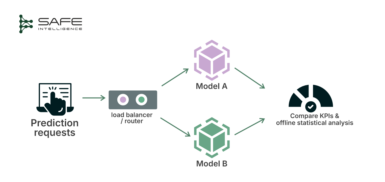
Why choose A/B testing?
It is primarily utilised in situations where it is ethically and operationally possible to treat different users differently for a brief period. For example, a bank might route a small percentage of transactions through a new fraud model to see if it catches more fraud or flags fewer false positives than the old model.
Flask-like pseudocode
TREATMENT_GROUP = set(load_user_ids_for_treatment())  # e.g., 10% users

@app.route("/predict")
def predict():
    data = request.get_json()
    features = data['features']
    user_id = data['user_id']

    # Determine if user is in treatment (B) or control (A) group
    if user_id in TREATMENT_GROUP:
        prediction = model_B.predict(features)
        variant = "B"
    else:
        prediction = model_A.predict(features)
        variant = "A"


    # Log results for offline statistically analysis
    log_ab_test_results(user_id, features, prediction, variant)

    return prediction
Scaling Your Deployment: Serving Hundreds or Thousands of ML Models
Once a single ML model delivers measurable business or safety improvements, rapid scaling becomes inevitable. Soon, you're managing not just a handful but hundreds or thousands of models, each bringing unique operational headaches, such as management complexity, resource contention, and cost efficiency. Leading enterprises, such as Netflix, have addressed these challenges using a proven framework: standardise, containerise, and orchestrate. Explore deeper insights:
Industry Best Practices: Serving Hundreds to Thousands of ML Models
TDS: Serve hundreds to thousands of ML models – architectures from industry
Actionable Takeaways
Pin down your performance requirements, resources, cost and scalability constraints, data dynamics and interactions early; these shape your deployment choices and downstream decisions.
Map your use case to the right pattern: real-time for instant results, async for flexible workloads, or batch for large-scale efficiency.
Rollout models progressively
Champion/Challenger: Safely validate a new model alongside the existing one without disruption.
Canary Deployments: Incrementally introduce new models, catching issues early and safely.
A/B Testing: Statistically validate model improvements on live traffic before full-scale deployment.
Standardise your configurations, containerise your models, and orchestrate your ML deployments. It’ll simplify complexity, reduce operational headaches, and make scaling frictionless.
Table of Contents
Rollout Strategies: Safely Deploying ML Models in Production
Scaling Your Deployment: Serving Hundreds or Thousands of ML Models